Adaptive Beamforming Tutorial Part 2: Preserving the Signal of Interest

Posted On January 11, 2020December 15, 2020 By Christopher Hogstrom

The Adaptive Beamforming Tutorial Parts 1 and 2 are available for download as a PDF!

Download The GrittyEngineer’s Guide to Adaptive Beamforing!

In Adaptive Beamforming Tutorial Part 1: Suppressing Interference we derived an adaptive nuller for a multi-element antenna that would attempt to suppress all signals detected above the noise floor. While a powerful tool, its use is limited to situations where the signal of interest (SOI) is below the noise floor. There are many cases where the SOI is detectable and we want to preserve the signal instead of crushing it. Even if the SOI is faint, adaptive beamforming can constructively combine the received signals to increase the SOI’s power while simultaneously mitigating interference.

There are numerous applications for this technology ranging from cochlear implants to self-driving cars, radio astronomy to submarines, and from 5G mobile phone technologies to military applications. More novel use cases are being explored and as antenna technology gets smaller and cheaper, many more will come in the future.

This tutorial is meant for engineers who are interested in understanding the math behind adaptive beamforming and might be interested in implementing an adaptive beamformer for their own application. We assume that you have already read Part 1 of this series and do not redefine our notation. However, Appendix A lists all of the variables used for easy reference.

Propagating Waves

Before we begin our discussion we need to understand some of the physics acting on our SOI. In many cases, we can assume that the SOI is generated by a point source and that the signal radiates equally in all directions. Imagine that the SOI is a sphere around the point source that grows larger the further it travels. If we were to take a small subsection of the imagined spherical SOI, say a square foot, while still close to the source we would see the small section greatly curved. However, taking a square foot subsection of the imagined spherical SOI a mile or two from the source would give us a section of the SOI that appears nearly planar. In fact, the curvature of the signal would probably be negligible for most applications and the signal would justifiably be assumed to be a plane wave. The point at which the curvature of the signal becomes negligible is called the far field (because you’re far away from the source). If the curvature of the signal is significant then you are in the near field (because you’re near the source).

For beamforming applications, the two biggest factors affecting whether you are in the near or far field are the distance between the source and the antenna, and the element spacing of the antenna array. The tighter the element spacing, the more likely you can assume being in the far field. However, there are tradeoffs between element spacing and performance that will not be discussed here. This adaptive beamforming tutorial assumes the antenna array is in the far field.

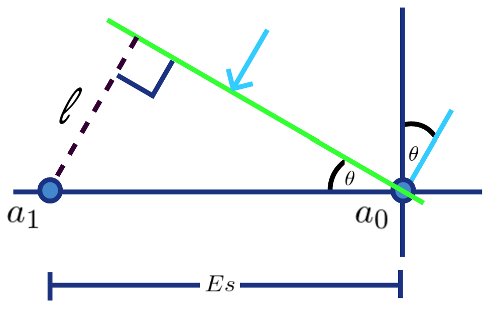
Figure 1 shows a simple line array where the distance between the antenna elements is $Es$ . Our signal of interest, the green planar wave, strikes the antenna with angle $\theta$ . Element $a_0$ receives the signal first and a short time later $a_1$ receives the signal. For narrowband signals, this time delay translates into a phase offset between the signal received at $a_0$ and $a_1$ . Determining the phase offset requires us to solve for $\ell$ using trigonometry. I still use the mnemonic SohCahToa to figure out which trigonometric formula to use. In this case, the hypotenuse and angle are known but the side opposite from the angle is not. Soh, or sine of theta equals opposite over hypotenuse will do the trick as shown below.

$\begin{align*} \sin(\theta) = \frac{\ell}{Es}\\ Es \sin(\theta) = \ell\\ \end{align*}$

Now we need to figure out how much the signal rotates traveling $\ell$ distance to $a_1$ . RF signals rotate a full $2\pi$ radians over the course of their wavelength which is written as, $\frac{2\pi}{\lambda}$ . If you’ve forgotten how to calculate the wavelength, $\lambda$ , check out the previous post. $\lambda$ has units of distance and it’s in the denominator of the fraction. We can simply multiply the equation just written by $\ell$ , which also has units of distance, to get our phase offset.

$\begin{align*} \phi &= \frac{2\pi}{\lambda} \ell\\ \phi &= \frac{2\pi}{\lambda} Es \sin(\theta)\\ \end{align*}$

Next, we write our steering vector $\mathbf{s}(\phi) = [1, e^{-j\phi}]^T$ . The steering vector simply contains the phase offsets the SOI experiences at each of the antenna elements with respect to $a_0$ . If we had N equally spaced antenna elements then our steering vector would be extended to $\mathbf{s}(\phi) = [1, e^{-j\phi},...,e^{-j(N-1)\phi}]$ .

Problem Setup

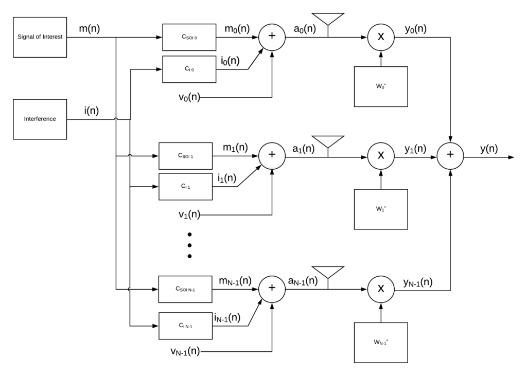
Figure 2 shows a block diagram of our system. The signal of interest, m(n), is the super-secret, ultra-important message you’re trying to receive. i(n) is the interference generated by the bad guys. C_{SOI p} is the channel response experienced by the SOI for antenna element p (includes things like delay, amplitude distortion, etc.), C_{I p} is the channel response experienced by the interference, v_p(n) is random white noise, a_p(n) is the received signal, W_p^* is the conjugate adaptive weight to rotate and scale the received signal, y_p(n) is the modified received signal and y(n) is the output of the system after the modified signals are summed together. Hopefully, you didn’t read that too fast and miss the fact that the weights, W_p, are conjugated which is different from what we’ve done in previous posts.

Mathematical Derivation

Our main objective is to minimize power while preserving the SOI. If this sounds like a constrained optimization problem then congratulations, your intuition is correct. Constrained optimization problems are composed of two parts, the cost function, $f(\mathbf{w})$ , that we want to either maximize or minimize and the constraint function, $c(\mathbf{w}) = g$ , that we must simultaneously satisfy. Previously, we learned that minimizing power is equivalent to minimizing $E\{|y(n)|^2\}= E\{|\mathbf{w}^H \mathbf{a}|^2\}$ where $\mathbf{y} = [a_0(n), a_1(n),\dots, a_{N-1}(n)]^T$ and $\mathbf{w} = [w_0, w_1,\dots, w_{N-1}]^T$ . This is our cost function. Preserving the SOI means that when the received signals are weighted and summed, signals originating in the direction of the SOI are undistorted. In other words, $\sum_{p = 0}^{N-1} w_p^*s_p(\phi) = 1$ or more succinctly, $\mathbf{w}^H\mathbf{s}(\phi)=1$ . This is our constraint function. We make one important assumption, that the SOI and the interference are uncorrelated i.e. $E\{m(n)i(n)^*\} = 0$ . Putting this all together we have

$\begin{align*}\underset{\mathbf{w}^H}{\arg\min}\{E\{|\mathbf{w}^H \mathbf{a}|^2\} \} \quad \text{s.t.} \quad \mathbf{w}^H \mathbf{s}(\phi) =1\\ \underset{\mathbf{w}^H}{\arg\min}\{E\{\mathbf{w}^H \mathbf{a}\mathbf{a}^H \mathbf{w}\} \} \quad \text{s.t.} \quad \mathbf{w}^H \mathbf{s}(\phi) =1\\ \underset{\mathbf{w}^H}{\arg\min}\{\mathbf{w}^H E\{\mathbf{a}\mathbf{a}^H \}\mathbf{w} \}\quad \text{s.t.} \quad \mathbf{w}^H \mathbf{s}(\phi) =1\\ \underset{\mathbf{w}^H}{\arg\min}\{\mathbf{w}^H \mathbf{R}_a\mathbf{w} \} \quad \text{s.t.} \quad \mathbf{w}^H \mathbf{s}(\phi) =1\\\end{align*}$

The cost function simplified to $w^H R_y w$ . We’ll use Lagrange multipliers to solve our constrained optimization problem. The first step is to create the Lagrangian function which combines the cost function and the constraint into a single equation while introducing the Lagrangian variable $\lambda$ .

$\begin{align*} h(\mathbf{w},\lambda) = f(\mathbf{w}) +\lambda(g-c(\mathbf{w}))\\ h(\mathbf{w},\lambda) = \mathbf{w}^H \mathbf{R}_a\mathbf{w} +\lambda(1-\mathbf{w}^H\mathbf{s}(\phi))\\ \end{align*}$

Minimizing $h(\mathbf{w},\lambda)$ is accomplished by taking the derivative with respect to $\mathbf{w}^*$ and setting it equal to zero.

$\begin{align*} \frac{\partial h(\mathbf{w},\lambda)}{\partial \mathbf{w}^*} = \mathbf{0} \\ \mathbf{R}_a\mathbf{w} -\lambda \mathbf{s}(\phi) = \mathbf{0}\\ \mathbf{R}_a \mathbf{w} = \lambda \mathbf{s}(\phi) \end{align*}$

(1) $\begin{align*} \mathbf{w} = \lambda \mathbf{R}_a^{-1}\mathbf{s}(\phi) \end{align*}$

Next, $\lambda$ is found by taking the derivative of the Lagrangian function with respect to $\lambda$ and setting it equal to zero.

$\begin{align*} \frac{\partial h(\mathbf{w},\lambda)}{\partial \lambda} = 0\\ 1-\mathbf{w}^H\mathbf{s}(\phi) = 0.\\ \end{align*}$

Substitute equation (1) for $\mathbf{w}$ and solve for $\lambda$ .

$\begin{align*} 1-(\lambda\mathbf{R}_a^{-1} \mathbf{s}(\phi))^H\mathbf{s}(\phi) = 0\\ 1-\lambda^* \mathbf{s}^H(\phi) \mathbf{R}_a^{-1}\mathbf{s}(\phi) = 0. \end{align*}$

Because $\mathbf{R}_a$ is Hermitian symmetric, $\mathbf{R}_a^{-1}$ is hermitian symmetric i.e. $(\mathbf{R}_a^{-1})^H = \mathbf{R}_a^{-1}$ .

$\begin{align*} \lambda^* \mathbf{s}^H(\phi) \mathbf{R}_a^{-1}\mathbf{s}(\phi) = 1\\ \end{align*}$

(2) $\begin{align*} \lambda^* = \frac{1}{ \mathbf{s}^H(\phi) \mathbf{R}_a^{-1}\mathbf{s}(\phi)}. \end{align*}$

The denominator of the fraction, $\mathbf{s}^H(\phi) \mathbf{R}_a^{-1}\mathbf{s}(\phi)$ , turns out to be a real only scalar. We won’t prove that out here but you can try generating a few hermitian symmetric matrices and multiplying them by a complex vector on the left and right side and see what you get. This means that $\lambda^* =\lambda$ and we can substitute (2) into (1) and finish solving for $\mathbf{w}$ .

(3) $\begin{align*} \mathbf{w} = \frac{\mathbf{R}_a^{-1}\mathbf{s}(\phi)}{ \mathbf{s}^H(\phi) \mathbf{R}_a^{-1}\mathbf{s}(\phi)} \end{align*}$

Beamformers with the solution found in (3) are called minimum variance distortionless response (MVDR) beamformers. The MVDR beamformer produces a distortionless response in the direction of the SOI thanks to the linear constraint placed earlier on the system, $\mathbf{w}^H\mathbf{s}(\phi)=1$ .

Now that we have the optimal weight vector, we can plug it back into our cost function $w^H R_y w$ and solve for the average power of the system.

$\begin{align*} \mathbf{w}^H\mathbf{R}_a\mathbf{w}\\ \left( \frac{\mathbf{R}_a^{-1}\mathbf{s}(\phi)}{ \mathbf{s}^H(\phi) \mathbf{R}_a^{-1}\mathbf{s}(\phi)}\right)^H \mathbf{R}_a \frac{\mathbf{R}_a^{-1}\mathbf{s}(\phi)}{ \mathbf{s}^H(\phi) \mathbf{R}_a^{-1}\mathbf{s}(\phi)}\\ \frac{\mathbf{s}(\phi)^H \cancel{\mathbf{R}_a^{-1}}}{ \mathbf{s}^H(\phi) \mathbf{R}_a^{-1}\mathbf{s}(\phi)} \cancel{\mathbf{R}_a} \frac{\mathbf{R}_a^{-1}\mathbf{s}(\phi)}{ \mathbf{s}^H(\phi) \mathbf{R}_a^{-1}\mathbf{s}(\phi)}\\ \frac{\cancel{\mathbf{s}(\phi)^H \mathbf{R}_a^{-1}\mathbf{s}(\phi)}}{\cancel{ \mathbf{s}^H(\phi) \mathbf{R}_a^{-1}\mathbf{s}(\phi)}} \frac{1}{ \mathbf{s}^H(\phi) \mathbf{R}_a^{-1}\mathbf{s}(\phi)}\\ \frac{1}{ \mathbf{s}^H(\phi) \mathbf{R}_a^{-1}\mathbf{s}(\phi)} \end{align*}$

Creating the Scanning Vector

Once we have solved for our weights, it’s common to look at the spatial response of our system. This means looking at the gain corresponding to different angles of arrival. To find the gain at different angles of arrival we generate steering vectors, now called scanning vectors because we are scanning the response, for each of the angles of interest. Then we take the dot product of our scanning vectors with our weights, i.e. $\mathbf{w}^H \mathbf{s}_\theta$ where $\theta$ is swept over all the angles of interest. Typically, the spatial response is visualized using either a two-dimensional plot for a uniform line array (ULA) or a heat map for a two-dimensional array of antenna elements.

To help visualize this I plotted the MVDR response for a six-element antenna system with inter-element spacing of $\lambda/2$ in Figure 3. The SOI impinges the antenna at $90^{\circ}$ while the interference impinges the antenna at $10 ^{\circ}$ . Notice that the gain in the direction of the SOI is 0 dB, corresponding to a gain of 1. Thus, our constraint was satisfied. Our interference, on the other hand, was pulled into a null. If you look closely though, the jammer is not in the absolute center of the null. The MVDR beamformer does not guarantee that the interference is placed in the absolute center of a null.

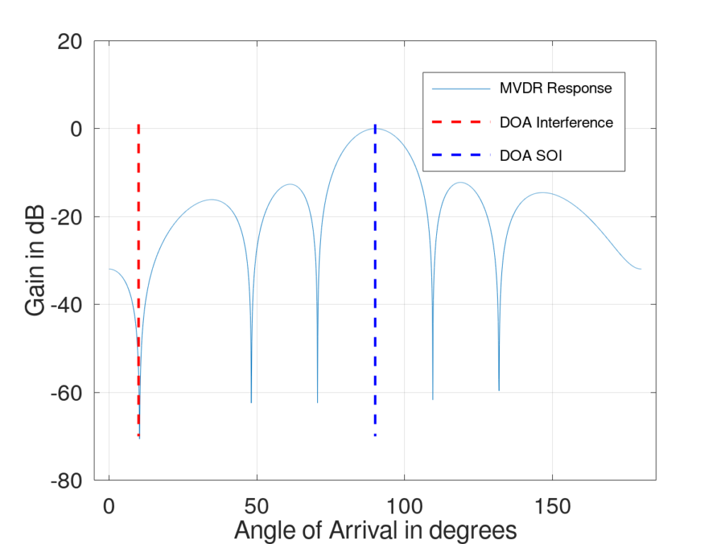
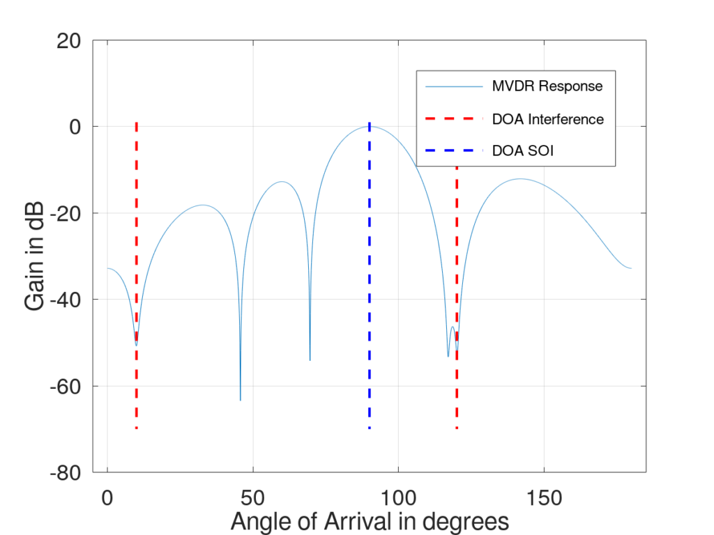
Figure 3: MVDR spatial response using a six-element antenna with an inter-element spacing of half a wavelength. Interference is at 10 degrees with SOI at 90 degrees.

Figure 4 shows the same setup but with an additional jammer at $120^{\circ}$ . Notice how the MDVR response adapted to the new interferer, hence the MVDR is an adaptive beamformer.

Figure 4: MVDR spatial response using a six-element antenna with an inter-element spacing of half a wavelength. Interference is at 10 degrees and 120 degrees with SOI at 90 degrees.

Conclusion

Adaptive beamformers are powerful tools. They can allow signals that are overwhelmed with interference to be successfully detected and processed. They allow you to digitally steer beams so if the SOI is moving the steering vector for the beamformer can be updated and you can track the SOI.

Though we did not cover it in this tutorial you can find the angle of arrival (AoA) of a signal using techniques like MUltiple SIgnal Classification (MUSIC) and Estimation of Signal Parameters via Rotational Invariance Technique (ESPRIT). This can be advantageous if you want to know the direction of your interferer.

Finally, the MVDR beamformer can be extended to the Linearly Constrained Minimum Beamformer (LCMV). LCMV generalizes the idea of placing constraints that the system must satisfy. For instance, maybe there are multiple signals you want to receive simultaneously but propagate from different directions. I’d love to hear your feedback in the comments section. If anything is unclear, just let me know and I’ll do my best to update this tutorial.

Appendix A: Variables defined

$\theta$	Propagating wave angle of arrival
$\ell$	Distance between propagating wave and antenna element
$Es$	Inter element antenna spacing
$\lambda$	Wavlength
$\phi$	Phase offset
$\mathbf{s}(\phi)$	Steering Vector. Contains the phase offsets the SOI experiences at each antenna element
$m(n)$	Signal of interest
$i(n)$	Interfering signal
$C_{SOI p}$	Channel response experienced by the SOI for antenna element $p$
$C_{I p}$	Channel response experienced by the interference for antenna element $p$
$v_p(n)$	Asynchronous white Gaussian noise (AWGN) on antenna element $p$
$a_p(n)$	Received signal at antenna element $p$
$W_p^*$	Optimal weight for element $p$ to minimize power while preserving SOI
$y_p(n)$	Weighted received signal from antenna element $p$
$y(n)$	System output after all $y_p(n)$ are summed
$\mathbf{R}_a$	Spatial correlation matrix of received samples

Christopher Hogstrom

christopher.hogstrom@grittyengineer.com

5 thoughts on “Adaptive Beamforming Tutorial Part 2: Preserving the Signal of Interest”

May says:

March 18, 2020 at 9:11 am

Thank you! Very helpful, and easy to understand

Reply
Tamiflu says:

July 15, 2020 at 3:46 am

Adaptive beamforming is a versatile approach to detect and estimate the signal-of interest at the output of a sensor array by means of data-adaptive spatial filtering and interference rejection. The object of this article is to link the adaptive beamforming capabilities to estimating algorithms from the ESPRIT family. To note that the simulated adaptive beamforming uses the estimation data received from the ESPRIT algorithms.

Reply
Sanj says:

October 22, 2020 at 10:55 pm

Thank you, that was very informative.

I had a question regarding adaptive beamforming, maybe you could help?
If I had a half-duplex phased array system on a spacecraft, and the spacecraft is tracking a ground station. If the spacecraft is using adaptive beamforming to track the ground station, and also transmit data to the ground station sequentially. I would think the spacecraft would lose the lock to ground station when it tries transmits, and would not be able to transmit at the ground station? Or is the the a way to follow the ground station without losing the lock during transmitting?

Thanks.

Reply
1. Christopher Hogstrom says:
  
  October 26, 2020 at 7:48 pm
  
  I think it depends on how the spacecraft is tracking the ground station. If it relies on the ground station’s transmission signal then I believe it would lose lock. However, if your spacecraft knows its precise location and orientation as well as the precise location of the ground station, then it can still form a beam in the direction of the ground station. Does that help?
  
  Reply
Bowen says:

August 29, 2022 at 3:18 am

The best MVDR beamformer tutorial I have ever seen!

Reply

Adaptive Beamforming Tutorial Part 2: Preserving the Signal of Interest

Propagating Waves

Problem Setup

Mathematical Derivation

Creating the Scanning Vector

Conclusion

Appendix A: Variables defined

5 thoughts on “Adaptive Beamforming Tutorial Part 2: Preserving the Signal of Interest”

Leave a Reply Cancel reply

Copyright All right reserved Theme: Multipurpose Business by Themeinwp

Blog

Propagating Waves

Problem Setup

Mathematical Derivation

Creating the Scanning Vector

Conclusion

Appendix A: Variables defined

Active Noise Cancellation with Multiple Auxiliary Sensors

The optimal Causal FIR Wiener filter

In the Top 75

5 thoughts on “Adaptive Beamforming Tutorial Part 2: Preserving the Signal of Interest”

Leave a Reply Cancel reply