Interpolation: The Advanced Game of Connect the Dots

**The Matlab code used for the examples is available for FREE at the end of the post**

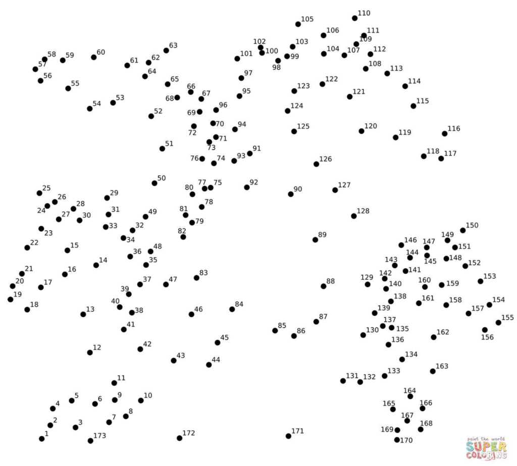
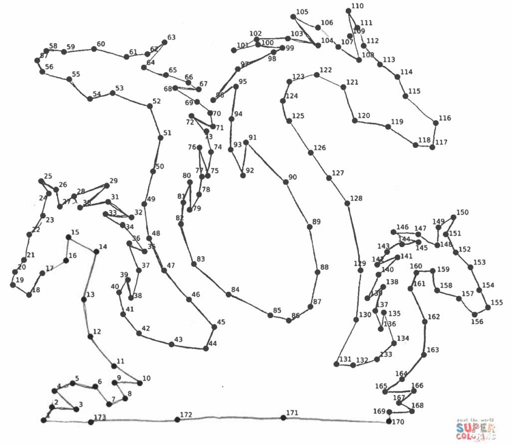
Every day thousands of kids across the world practice interpolation, and they do it for fun. The best part, they don’t even know it’s called interpolation to them it’s just a game called Connect-the-Dots. You might remember it from your childhood. A teacher or parent would give you a white sheet of paper filled with dots numbered 1 to N, like the one shown in Figure 1 (thanks supercoloring.com). The goal is to recreate the image by sequentially connecting the dots. The children typically connect the dots in the most efficient manner by using a straight line. Once all the dots are connected, it’s easy to see the original image as demonstrated in Figure 2.

Figure 1: Example Connect the Dots worksheet.

Linear interpolation example — Figure 2: Completed connect the dots worksheet.

What is Interpolation?

Interpolation is the process of estimating data between two or more samples. The dots in a Connect-the-Dots game can be viewed as samples taken from an illustration’s outline. The straight line drawn between two points represents an estimate of the missing data. This post lists several different interpolation methods and some of their applications.

Linear Interpolation

Linear interpolation uses two samples to estimate the missing data by finding the line that intersects both points. The missing data is estimated to be on the line. The children in the opening example use linear interpolation to great effect. The equation for linear interpolation can easily be derived from the equation of a line (expand the hidden text if interested) and is

The equation of a line is

$\begin{align*} y = mx+b. \end{align*}$

The first step is to solve for $m$ and $b$ which can be accomplished by using the samples before and after the desired interpolated sample.

$\begin{align*} y_0 &= m x_0 + b\\ y_1 &= m x_1 + b\\ \end{align*}$

Because this is a system of equations we can use linear algebra to put it in matrix form.

$\begin{align*} \begin{bmatrix} y_0\\ y_1 \end{bmatrix} = \begin{bmatrix} x_0 & 1\\ x_1 & 1 \end{bmatrix} \begin{bmatrix} m\\ b \end{bmatrix} \end{align*}$

Next we find the inverse of our 2×2 matrix and multiply it on the to the left hand side of the equation

$\begin{align*} \frac{1}{x_0-x_1} \begin{bmatrix} 1 & -1 \\ -x_1 & x_0 \end{bmatrix} \begin{bmatrix} y_0\\ y_1 \end{bmatrix} &= \begin{bmatrix} m\\ b \end{bmatrix}\\ \frac{1}{x_0-x_1} \begin{bmatrix} y_0 - y_1\\ -y_0 x_1 + y_1 x_0 \end{bmatrix} &= \begin{bmatrix} m\\ b \end{bmatrix} \\ \begin{bmatrix} \frac{y_0-y_1}{x_0-x_1}\\ \frac{-y_0 x_1 + y_1 x_0}{x_0-x_1}\\ \end{bmatrix} &= \begin{bmatrix} m\\ b \end{bmatrix} \end{align*}$

Before we move on, let’s decompose $x_1$ . It is assumed that our signal of interest has been sampled at some constant rate $T$ . Thus $x_1$ can be re written as

$\begin{align*} x_1 = x_0 + T. \end{align*}$

Substituting $x_0+T$ for $x_1$ in our equation for $m$ and $b$ results in

$\begin{align*} \begin{bmatrix} \frac{y_0-y_1}{-T}\\ \frac{-y_0 x_1 + y_1 x_0}{-T} \end{bmatrix} = \begin{bmatrix} m\\ b \end{bmatrix} \end{align*}$

Now we can find $y_{\mu}$ by

$\begin{align*} y_{\mu} = \frac{y_0 - y_1}{-T} x_{\mu} + \frac{-y_0 x_1 + y_1 x_0}{-T} \end{align*}$

However, just like $x_1$ was re written in terms of $x_0$ we can also re write $x_{\mu}$ in terms of $x_0$ as follows

$\begin{align*} x_{\mu} = x_0 + \mu T. \end{align*}$

Substituting this in we get

$\begin{align*} y_{\mu} &= \frac{1}{-T}((y_0-y_1)(x_0+\mu T) - y_0(x_0+T)+y_1x_0)\\ &= \frac{1}{-T}(y_0 x_0 + y_0 \mu T - y_1x_0 -y_1 \mu T - y_0 x_0 -y_0T + y_1_x_0)\\ \end{align*}$

Next, we simplify.

$\begin{align*} &= \frac{1}{-T}(y_0 \mu T - y_1 \mu T - y_0 T)\\ &= y_1 \mu -y_0 \mu +y_0\\ &= \mu y_1 + (1-\mu) y_0 \end{align*}$

$\begin{align*} y_{\mu} = \mu y_1 + (1-\mu)y_0 \end{align*}$

where $y_{\mu}$ is the interpolated value and $\mu$ is the fractional sample time. There are a couple of important observations. First, $y_{\mu}$ is the output of a linear combination of samples i.e. the input samples are only scaled and added instead of being raised to some power. As such, $y_{\mu}$ can be considered the output of a linear low-pass filter who’s coefficients are $\mu$ and $1-\mu$ . Second, the filter coefficients are dependent on the desired sampling instant, not the sample themselves. If the desired sampling instant does not change, then the coefficients themselves remain the same.

The above equation finds a single interpolated value but there are many occasions where you want a higher resolution data-set. We accomplish this by upsampling (inserting zeros in between samples) and low-pass filtering. The low-pass filter is found by sweeping the desired sampling instant and computing the filter coefficients. For example, suppose we wish to upsample our data-set by four. We’d insert 3 zeros in between all of the samples and sweep $\mu$ from $0$ to $1$ in $\frac{1}{4} = 0.25$ increments as shown in Table 1.

$\mu$	$1-\mu$
0	1
0.25	0.75
0.5	0.5
0.75	0.25
1	0

Table 1:Linear interpolation coefficients for swept $\mu$ at 0.25 increments.

By offsetting the filter coefficients by the desired interpolant’s index (0,1,2,3 or 4) and combining them, we get the upsampled, linear interpolation filter shown in Figure 3.

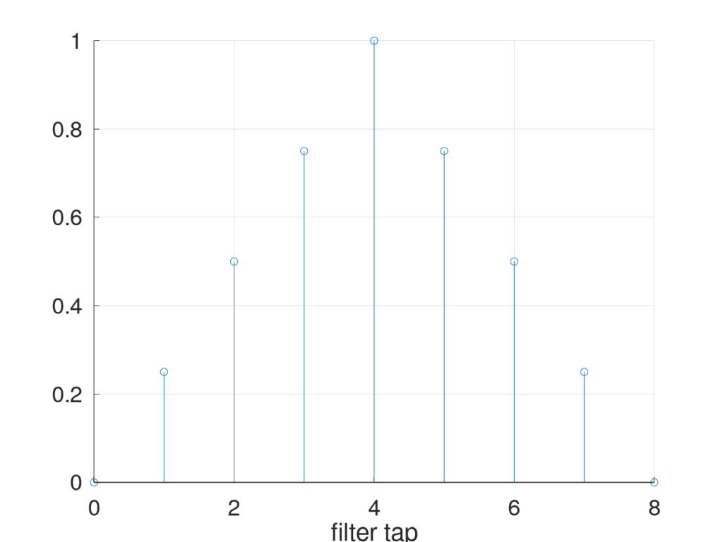
Figure 3: Upsampled linear interpolation filter.

This filter can now be used on the upsampled data set.

Linear interpolation short cut

Instead of using the equation above to compute the filter coefficients, you could instead create the triangular filter by convolving two rects. Personally, this is my preferred method and can be accomplished by following the steps below.

Upsample your data using an integer factor N.
Create a rect whose width is the same as the upsample factor e.g. if your upsample factor is four create a rect that is four taps wide
Convolve the rect with itself to create your trianlge pulse. This will produce a triangle pulse that is 2*N-1 taps wide
Scale the triangle pulse so that the largest tap is one.
Filter your upsampled data from step one with your triangle pulse.

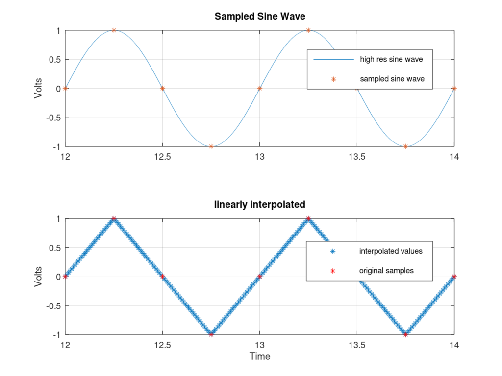
Figure 4 illustrates linear interpolation on a sine wave. The top plot is a sine wave sampled at two times the Nyquist sampling rate where the red asterisks represent the samples. The bottom plot is the linearly interpolated approximation to the sine wave only using the red samples. As you can see, linear interpolation didn’t render the most accurate results.

Figure 4: (Top) High res sine wave sampled at the red asterisks. (Bottom) Sine wave approximation using linear interpolating filter.

Linear Interpolator Use case

Linear interpolation is simple and computationally easy. It’s great when only coarse approximations are needed or if your signal is already highly oversampled. It’s extremely quick and uses the fewest number of samples. That being said, for many applications, linear interpolation doesn’t produce accurate enough measurements.

Piecewise Polynomial Interpolation

Piecewise Polynomial interpolation is similar to linear interpolation, in fact, linear interpolation just a specific form of piecewise polynomial interpolation. The difference is instead of using a 1st-degree polynomial (linear) to estimate the missing data you use an N-degree polynomial. However, odd degrees are by far the most common with 3rd-degree polynomials being the most common (also known as cubic interpolators). This is because odd degreed polynomials use an even number of samples to solve for the unknowns, allowing for half of the samples used to come before the desired interpolation point and half coming after the desired interpolation point. Because cubic interpolators are so common, we’ll show what that looks like. The equation for a cubic polynomial is

$\begin{align*} y = ax^3 +bx^2+cx+d \end{align*}$

Notice there are four unknowns, $a$ , $b$ , $c$ , and $d$ . The problem set up is the same for the linear interpolation shown earlier. Because inverting a 4×4 matrix is much more difficult and time-consuming, I’m just going to skip it all and give you the equation to find an interpolated value using a cubic interpolator.

$\begin{align*} y_{\mu}=&\left(\frac{\mu^3}{6}-\frac{\mu}{6}\right) y_2\\ -&\left(\frac{\mu^3}{2}-\frac{\mu^2}{2}-\mu\right) y_1\\ +&\left(\frac{\mu^3}{2}-\mu^2-\frac{\mu}{2}+1\right) y_0\\ -&\left(\frac{\mu^3}{6}-\frac{\mu^2}{2}-\frac{\mu}{3}\right) y_{-1} \end{align*}$

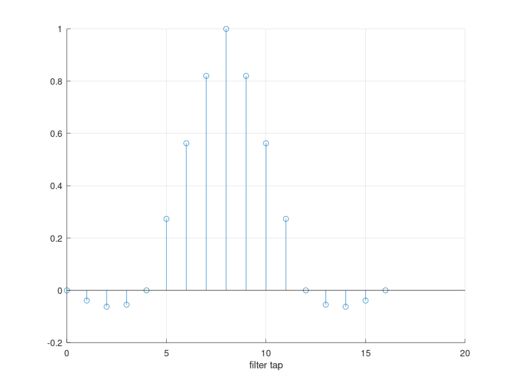
Just as with the linear interpolator, the cubic interpolator can be viewed as a low pass filter whose filter coefficients are the terms multiplying the $x$ s. Sweeping $\mu$ from $0$ to $1$ in $0.25$ increments creates filter response (filter coefficients for signal upsampled by 4) shown in Figure 5.

Figure 5: Cubic interpolation filter coefficients for an upsample by 4.

As an example, I have taken a low resolution sampled sine wave, upsampled it by 30, and applied the corresponding cubic interpolation filter. The results are shown in figure 6.

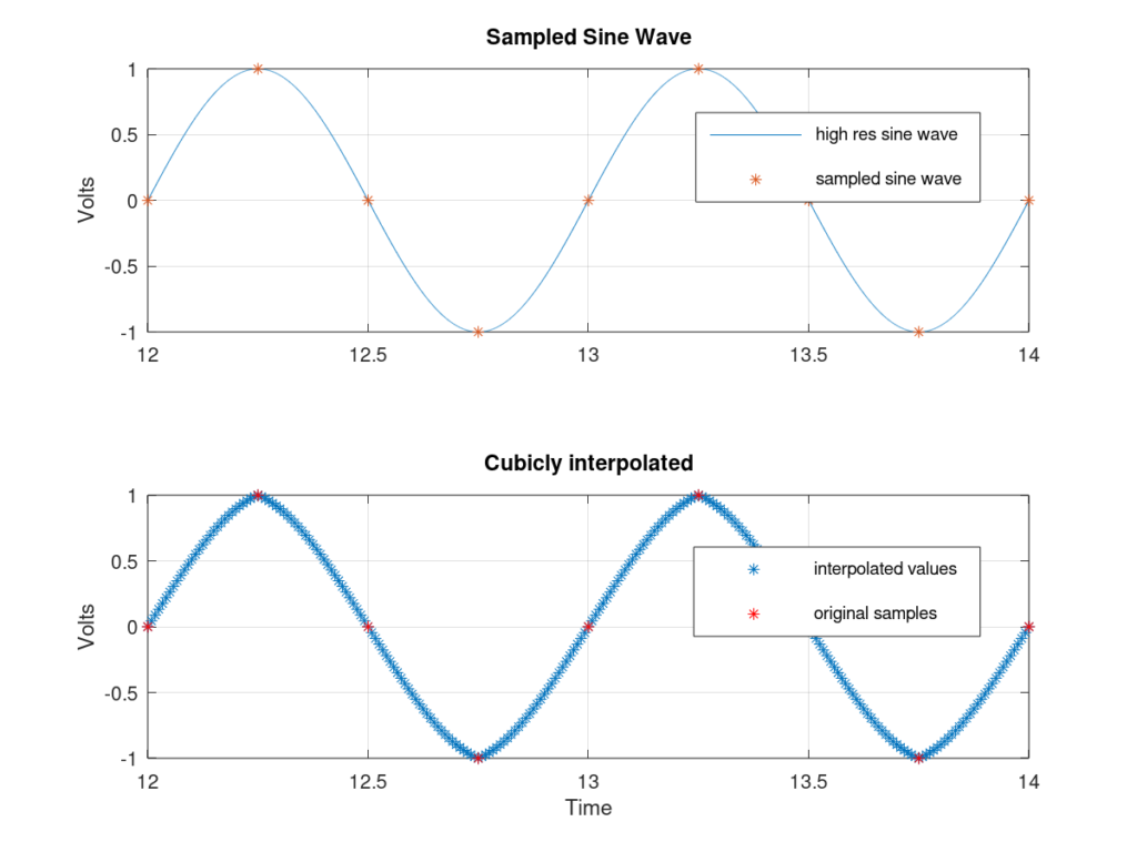
Figure 6: (Top) High res sine wave sampled at the red asterisks. (Bottom) Sine wave approximation using cubic interpolating filter.

As can be seen from the figure, the cubic interpolator does a better job of approximating the sine wave. You can see that the points are rounded, unlike the linear approximation. Obviously, this still isn’t a very good approximation but for some applications, this works well. As you might have guessed, if you wanted a better approximation to the sine wave, you could keep increasing the polynomial degree i.e. use a 5th or 9th-degree polynomial.

Piecewise Polynomial Interpolator Use Case

Transmitters contain a local oscillator that mixes a baseband signal to the correct center frequency. Receivers also contain a local oscillator to mix the received signal down back to baseband. However, because we live in the real world, the oscillators are not at exactly the same frequency. They’ll be close to each other but not perfectly the same. As a result, the samples generated by the analog to digital converter (ADC) are almost never at the desired sampling instant. Luckily we can do some clever math to find the optimal sampling instant and then use cubic interpolation, or a higher-order polynomial filter, to find the desired sample.

Windowed Sinc Interpolation

So what is the best interpolating filter? The answer, derived from sampling theory (which is beyond the scope of this post), is the sinc interpolator. In fact, for a band-limited signal (assuming the signal was sampled at Nyquist) a sinc interpolator would perfectly recreate the original signal. So why don’t we just use a sinc interpolator? Well, for a few reasons. The equation for the sinc function is

$\begin{align*} \text{sinc} = \frac{\sin(x)}{x} \end{align*}$

where $x$ extends from $-\inf$ to $+\inf$ . As far as I know, no computing device has been made that can compute an infinite number of points for a given filter. Furthermore, most real-life data sets we want to analyze have a starting or ending point. Thus using the perfect sinc interpolator is physically impossible.

However, instead of trying to do the impossible, you could just truncate the function after it has sufficiently approached zero. Depending on the application, that might still require more samples than we wish. The other option is to truncate the sinc function and then apply a window to it so that spectral leakage is minimized. The post on DSP Related, found here, does a really good job of explaining this concept.

Using a windowed sinc is actually pretty easy to do. The first step is to sample the sinc function at one over the upsample factor i.e. $\frac{1}{upSampFac}$ . The next step is to take your favorite window and apply it to the sampled sinc function. I’ve shown the results of this in Figure 7.

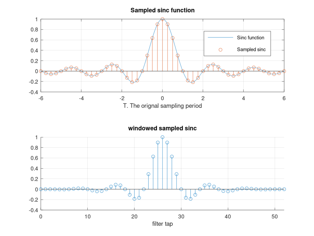
Figure 7: (Top) Sinc function sampled at 1/4. Notice the x-axis is in the sample rate T (Bottom) Windowed sinc filter using a Hann window. Notice x-axis has been converted to filter tap.

The next step is to convolve the upsampled data set with the windowed sinc filter. I’ve shown the results of doing this in Figure 8. Here the upsample factor is 30 and I’ve selected 6 zero crossings for my sinc interpolator. As can be clearly seen, the sinc interpolator almost perfectly reproduces the sampled sine wave.

Figure: 8 (Top) High res sine wave sampled at the red asterisks. (Bottom) Sine wave approximation using windowed sinc interpolating filter.

Windowed Sinc Interpolator Use Case

Windowed sinc interpolators commonly find applications in fractional delay filters. Such filters are used when the data set needs to be delayed by a fraction of the sample rate. For example, the delay & sum time-domain adaptive beamformer works by carefully delaying the received signals from multiple antennas. The amount each signal is delayed will differ from one signal to the next and will almost always be some fraction of the sampling rate. Thus a windowed sinc interpolator is needed. After appropriately delaying the signals, the signals are added together, creating nulls and gains in desired directions. See here for more info on adaptive beamformers.

Fourier-based interpolation

Chad Spooner from the cyclostationary.blog website, suggested that we include a Fourier based method of interpolation. Fourier-based interpolation is a pretty cool idea. We know that zero padding a signal in the time-domain results in an increased sample rate in the frequency-domain. Conversely, by zero padding in the frequency domain, we are increasing the sample rate in the time-domain.

Interpolation using the Fourier-based method can be accomplished by the following steps:

Transform the original time-domain signal to the Fourier-domain using an N point FFT where N is the of data samples.
Insert N*(L-1) zeros in the middle of the Fourier-domain dataset
- L is the upsample factor
Apply an N*L inverse FFT on the upsampled Fourier-domain dataset
Scale the new time-domain signal by L

The last step, scaling by the upsample factor, is needed because the energy contained in the signal is spread across more points.

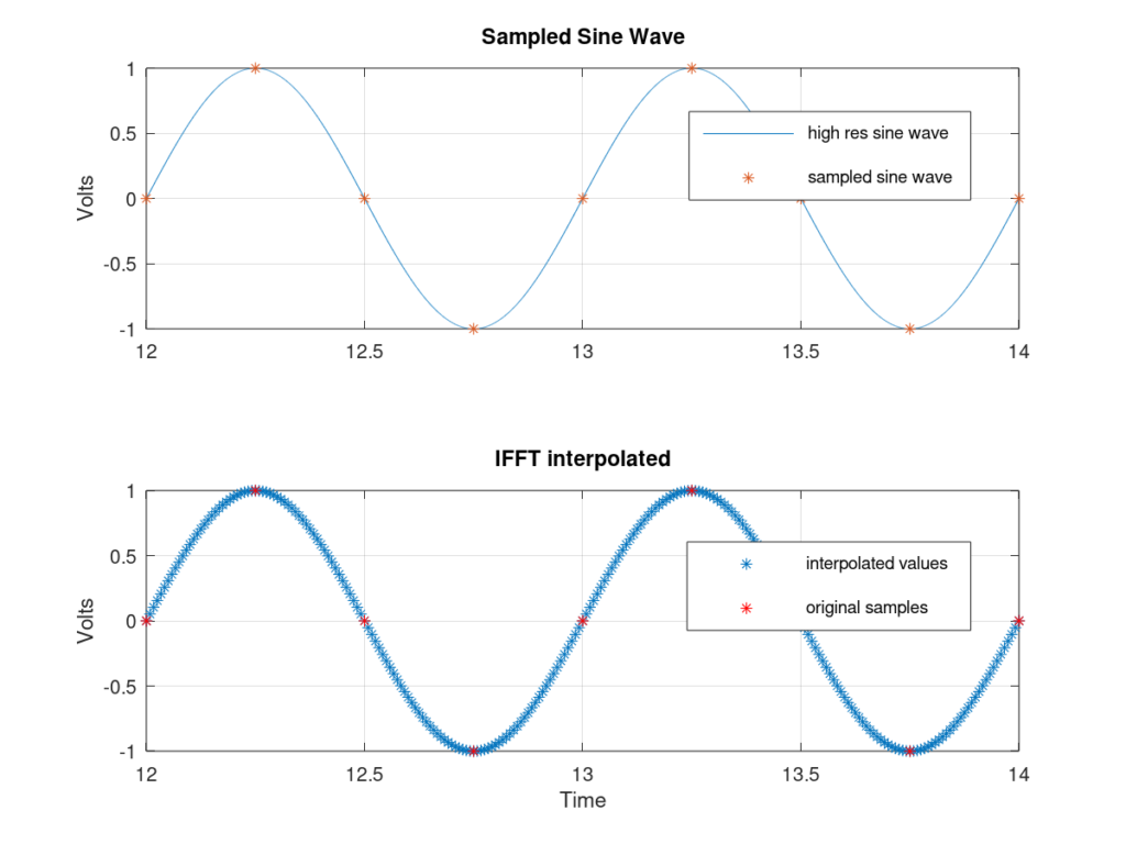
An example of zero padding is shown in Figure 9. The top plot shows the FFT for the original dataset sampled at 4 Hz (the same dataset shown on the top plot of Figure 10). Note that the x axis is the index of the frequency-domain values without doing an fftshift. This is the output when performing Octave’s or Matlab’s FFT function.

The second step is shown in the bottom plot of Figure 9. Here the frequency-domain data has been zero-padded in the middle. It’s important that the dataset remain symmetric.

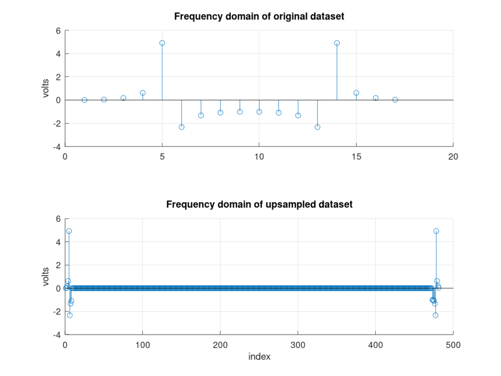
Figure 9: (Top) FFT of original dataset sampled at 4 Hz. (Bottom) Upsampled frequency domain by a factor of 30.

Finally, the last two steps are to take the inverse FFT of the upsampled frequency-domain dataset and scale by the upsample factor, the results of which are shown in Figure 10. Notice that the approximation is similar to the windowed sinc interpolation.

Figure 10: (Top) High res sine wave sampled at the red asterisks. (Bottom) Sine wave approximation using Fourier-based interpolation.

Fourier-based Interpolator Use Case

The time-domain based interpolation methods mentioned above all allow for streaming-based processing. In other words, as a new upsampled value comes in, a new value is interpolated. However, with the Fourier-domain interpolation method described above a block processing approach must be taken. This means buffering N samples before interpolating, requiring more memory. Some applications do not require real-time operation and can handle the increased latency. The advantage is very accurate interpolations. And if N is a power of 2 you can take advantage of highly optimized algorithms.

One thing to note, the discrete Fourier transform expects the signal to be exactly periodic over the number of samples used in the transform. If it is not exactly periodic, you will see Gibbs’ phenomenon produce errors at the beginning and ending of the interpolated values.

Conclusion

This post has gone over the most basic interpolators, there are many others. Interpolators are used in many digital signal processing applications and should be something every DSP engineer is familiar with. So, whether you are computing the optimal sample for a receiver or you are delaying a signal in time, it’s all about connecting the dots.

Send me the free code!

Interpolation: The Advanced Game of Connect the Dots

What is Interpolation?

Linear Interpolation

Linear interpolation short cut

Linear Interpolator Use case

Piecewise Polynomial Interpolation

Piecewise Polynomial Interpolator Use Case

Windowed Sinc Interpolation

Windowed Sinc Interpolator Use Case

Fourier-based interpolation

Fourier-based Interpolator Use Case

Conclusion

One thought on “Interpolation: The Advanced Game of Connect the Dots”

Leave a Reply Cancel reply

Copyright All right reserved Theme: Multipurpose Business by Themeinwp

Blog

What is Interpolation?

Linear Interpolation

Linear interpolation short cut

Linear Interpolator Use case

Piecewise Polynomial Interpolation

Piecewise Polynomial Interpolator Use Case

Windowed Sinc Interpolation

Windowed Sinc Interpolator Use Case

Fourier-based interpolation

Fourier-based Interpolator Use Case

Conclusion

In the Top 75

Adaptive Beamforming Tutorial Part 2: Preserving the Signal of Interest

One thought on “Interpolation: The Advanced Game of Connect the Dots”

Leave a Reply Cancel reply