Adaptive Beamforming Tutorial Part 1: Suppressing Interference

In Active Noise Cancellation with Multiple Auxiliary Sensors we left off with the question, “How can we mitigate interference when all of our sensors receive the signal of interest and interference?” Part 1 of this adaptive beamforming tutorial explains how to suppress the interference and lays the foundation to steer gain to specific locations.

An array of antennas that can be used for adaptive beamforming.

Sine Wave Fundamentals

Let’s talk about good old sine waves for a moment. Sine waves are represented by the equation

$y(t) = A \sin(\omega t + \theta)$

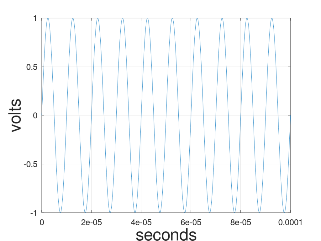
where $A$ is the amplitude, $\omega$ is the frequency in radians, $t$ is time, and $\theta$ is the phase. Often when we talk about sine waves we look at a signal and how it varies across time. Figure 1 shows a simple 100k Hz radio frequency (RF) sine wave. An RF antenna receives this signal and an analog to digital converter (ADC) samples the signal in time. In this case, we have fixed the spatial location of the sensor but allow time to vary in order to capture the sine wave.

Now let’s imagine for a moment that we are powerful wizards with the ability to freeze time. With time frozen, we sample the signal through space. Interestingly, a sine wave sampled in space still looks like a sine wave. The x-axis changes from time to distance but the units on the y-axis remain the same. The distance a sine wave travels before completing a full period is called a wavelength. Finding the wavelength is relatively easy as long as we know two things, the frequency of the sine wave and the speed at which it propagates through our desired medium. RF signals travel at the speed of light in free space (a vacuum) which is about 3e8 $\frac{meters}{sec}$ . Hz is in units $\frac{cycles}{sec}$ and wavelengths are in units $\frac{meters}{cycle}$ . To get wavelengths simply multiply the propagation speed by the reciprocal of the frequency as shown below.

$\begin{align*} \frac{3e8 meters}{1 sec} *\frac{1 sec}{100e3 cycles} = 3e5 \frac{meters}{cycle}.\\ \end{align*}$

Figure 2 plots the wavelength for our 100k Hz signal.

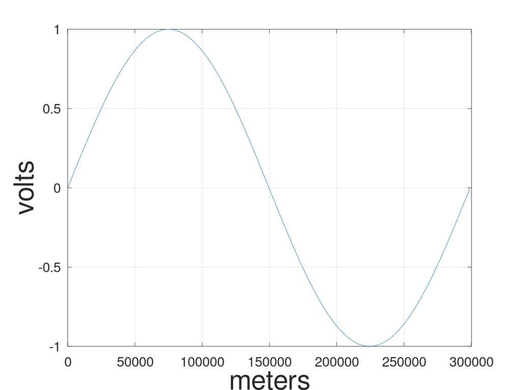
Figure 2: 100K Hz RF wavelength through free space.

If we put a sensor on the x-axis at location zero and another sensor on the x-axis at a quarter wavelength away, at 75,000 meters in the direction of propagation, the phase difference between the two would be 90 degrees. Leaving the two sensors at zero and at a quarter wavelength away (we’ll call them sensor a and b respectively), we can unfreeze time and get two sine waves with a 90-degree phase offset as shown in Figure 3.

Figure 3: Blue plot is the signal received from sensor a. Blue dashed plot is the signal received from sensor b.

Here’s where it gets exciting, we can apply a phase offset to our captured signals so that when the signals are added together they either add constructively or destructively. For example, rotating signal b by -90 degrees and adding it to signal a amplifies the received signal as shown in Figure 4. On the other hand, rotating signal b by 90 degrees and adding it to signal a cancels out the received signal as shown in Figure 5.

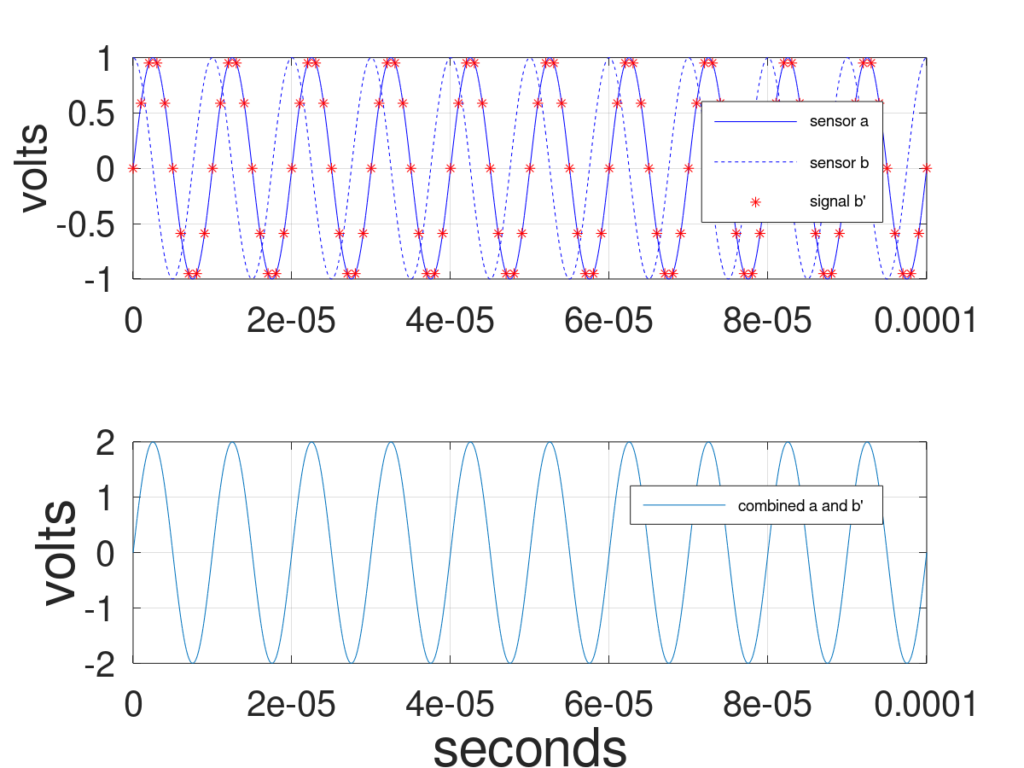
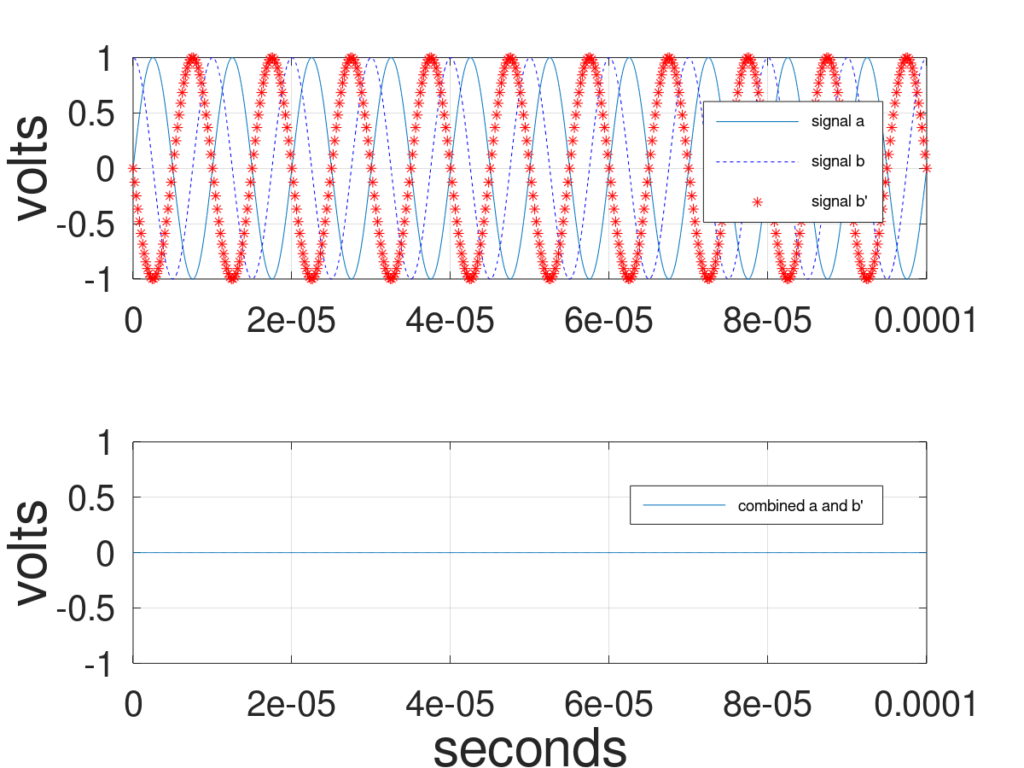
Constructive sine wave addition for adaptive beamforming tutorial. — Figure 4: Top shows signal captured by sensor a in blue, signal captured by sensor b as blue dashed, and rotated b as asterisks. Bottom plot is the combined a and rotated b signal.

Sine wave cancellation for adaptive beamforming tutorial. — Figure 5: Top shows signal captured by sensor a in blue, signal captured by sensor b as blue dashed, and rotated b as asterisks. Bottom plot is the combined a and rotated b signal.

This adaptive beamforming tutorial relies on the ability to shift and scale received signals so that they add constructively or destructively.

An alternate representation of Sine waves

Sine waves can also be represented using complex notation as follows

$y(t) = A e^{j (\omega t+\theta)}$

where $A$ is the amplitude of the sine wave, $j$ is the imaginary number, $\omega$ is the frequency in radians, and $\theta$ is the phase. Beamformers typically use complex numbers to represent signals because rotating a complex sine wave is accomplished by multiplying the signal by the complex number $e^{j \phi}$ where $\phi$ is the desired phase offset.

However, transmitters emit real-valued signals, not complex signals which means that signals have both positive frequency and negative frequency components. The positive and negative frequency components are symmetric and therefore redundant. In contrast, complex-valued signals are not symmetric meaning that the positive and negative frequency components provide unique and useful information. New engineers often ask, “How do we convert our real-valued signals into complex signals?”

Most systems employ one of two methods for obtaining the complex-valued signals. The first is to sample the real-valued signals using ADCs, then use a Hilbert transform to convert the real-valued samples to complex-valued samples. The Hilbert transform suppresses the negative frequency components of the signal. More information about the Hilbert transform can be found here. The second method employs a technique called quadrature sampling. Quadrature sampling creates complex samples at the ADC and avoids the necessity of using the Hilbert filter. A great tutorial on quadrature sampling can be found here.

A Use Case for Adaptive Beamforming

Let’s say that you and your team are trying to receive a super-secret, ultra-important message that’s transmitted using spread-spectrum techniques. Because this message is so secret (it’s about a brand new breed of dogs that forever looks like puppies), the signal is transmitted below the noise floor to avoid detection by nefarious groups (this is the same technique employed by most satellite downlinks, Bluetooth, and many military communication systems. The receiver performs long integration to bring the signal above the noise floor). While the trouble makers can’t detect the signal themselves, they know what frequency your signal is on and are trying to create interference so that you can’t get the information either. This interference is well above the noise floor and easily detected.

Luckily you’ve been reading this adaptive beamforming tutorial and know that you can rotate and combine signals sampled in space to cancel interference. You and your team decide to place three sensors in an equilateral triangle formation where the distance between any two sensors is a half wavelength.

Figure 6 shows a block diagram with the setup you’re most likely to encounter. The signal of interest, s(n), is the super-secret, ultra-important message you’re trying to receive. i(n) is the interference generated by the bad guys. C_{SOI p} is the channel response experienced by the signal of interest (SOI) for antenna element p (includes things like delay, amplitude distortion, etc.), C_{I p} is the channel response experienced by the interference, v_p(n) is random white noise, a_p(n) is the received signal, W_p is the adaptive weight to rotate and scale the received signal, y_p(n) is the modified received signal and y(n) is the output of the system after the modified signals are summed together.

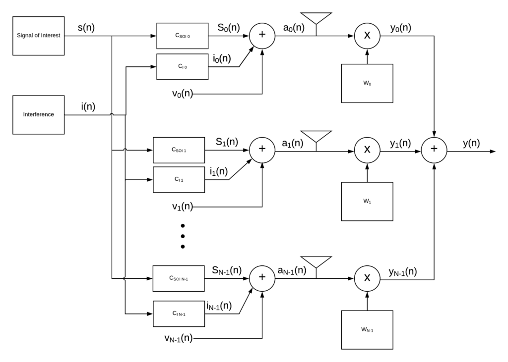
Figure 6: Block diagram of a narrowband beamformer.

In this adaptive beamforming tutorial, we’re going to take advantage of the fact that the SOI is below the noise floor and create an adaptive nuller. An adaptive nuller places spatial nulls in the direction of greatest power but does not constrain the weights to create spatial gain in any particular direction. Because our SOI is below the noise floor, the nuller can’t sense it and won’t intentionally attenuate the SOI signal. Placing spatial gains (forming beams in specific directions) will be covered in part two of this tutorial and is a natural extension of what we’ll learn here.

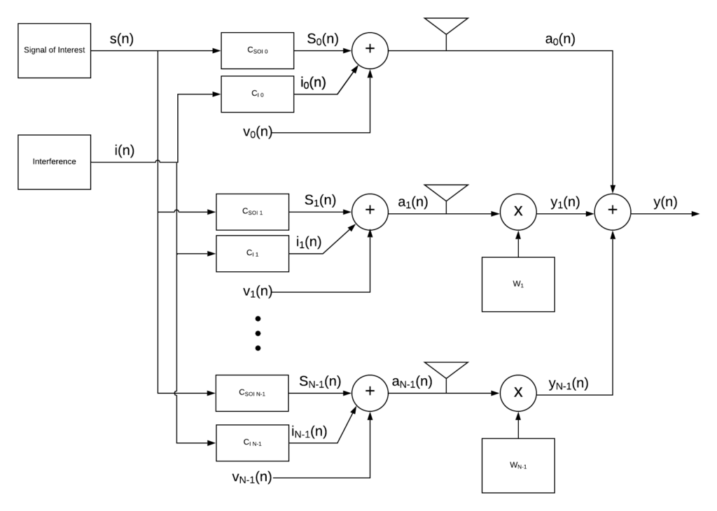
Leveraging the fact that the SOI is below the noise floor, our goal is to minimize the output power $E\{y(n)^2\}$ . However, if we minimize the output using the block diagram in Figure 6 the solution to our weights will be zero. After all, how could you have less power than nothing at all? To avoid this, we let one of our antenna elements be the reference sensor. The signal captured by the reference element passes through unmodified (essentially setting the weight for that element to one) as shown in Figure 7.

Figure 7: Block diagram of narrowband nuller where element one is the reference element.

Post Notations

Before going on to the derivation, let’s define some notation so that we’re all on the same page. Let $E\{\cdot\}$ , $\hat{d}$ and $r_d(k)$ represent the expectation operator, the estimate of $d$ , and the autocorrelation function of $d$ respectively. The expectation operator returns the expected value or mean of a random variable.

The signal $y$ is found by combining the filtered auxiliary signals $y_q$ where $0<q< N$ . $y_q$ is found by multiplying $a_q$ with our optimal weights as follows

$y_q(n) = w_q a_q$

where $p$ is the antenna element.

The autocorrelation function for a wide sense stationary (WSS) signal is defined as

$r_v(k) = E\{v(n)v^*(n-k)\}$

where $n$ is the current sample and $k$ is an integer offset. The cross-correlation function for jointly WSS signals is defined as

$r_{v_1 v_2} = E\{v_1(n)v_2^*(n-k)\}$

Let the power of the signal be defined as

$\zeta = E\{y(n)^2\}$ .

Finally, let $\cdot^*$ represent the complex conjugate operator.

Adaptive Nulling Derivation

As stated previously, nullers minimize output power with respect to the weights. Mathematically, the equation looks like

$\begin{align*} \text{argmin} \{E\{y(n)^2\}\} \quad \text{with respect to } w_q^*.\\ \end{align*}$

Making a few substitutions we get

$\begin{align*} \text{argmin} \{E\{(a_0 + \sum^{N-1}_{p = 1} y_p)^2\}\}\\ \text{argmin} \{E\{(a_0 + \sum^{N-1}_{p = 1}a_{p} w_{p})^2\}\}.\\ \end{align*}$

Because the above equation is quadratic and differentiable everywhere, finding the minimum is relatively easy. Simply take the derivative with respect to the weight we are solving for and set it equal to zero.

$\begin{align*} \frac{\partial}{\partial w_q^*}E\{(a_0 + \sum^{N-1}_{p = 1}a_{p} w_p)^2\}=0\\ E\{(a_0 + \sum^{N-1}_{p = 1}a_{p} w_p)a_q^*\}=0\\ E\{a_0a_q^* + \sum^{N-1}_{p = 1}a_{p}a_q^* w_p\}=0\\ E\{a_0a_q^*\} + \sum^{N-1}_{p = 1}E\{a_{p}a_q^* \}w_p=0\\ r_{a_0 a_q} +\sum^{N-1}_{p = 1}r_{a_p a_q }w_p=0\\ \sum^{N-1}_{p = 1}r_{a_p a_q }w_p=-r_{a_0 a_q} \\ \end{align*}$

The above equation is generic for solving for each of the weights where $0<q<N$ . You’ll commonly see systems of equations like this represented in matrix-vector form as shown below.

$\begin{align*} \mathbf{R}\mathbf{w} = -\mathbf{r}\\ \end{align*}$

where

$\begin{align*} \mathbf{R} = \begin{bmatrix}\mathbf{r}_{a_1 a_1} & \dots & \mathbf{r}_{a_{N-1} a_1}\\\vdots & \vdots & \vdots\\\mathbf{r}_{a_1 a_{N-1}} &\dots & \mathbf{r}_{a_{N-1} a_{N-1}}\\\end{bmatrix},\\ \mathbf{w} = \begin{bmatrix}w_1\\\vdots\\w_{N-1}\end{bmatrix},\\ \end{align*}$

and

$\begin{align*} \mathbf{r} = \begin{bmatrix} r_{a_0 a_1}\\ \vdots\\ r_{a_0 a_{N-1}}\\ \end{bmatrix}\\ \end{align*}$

Some adaptive beamforming tutorials will call $\mathbf{R}$ a covariance matrix. Do not be fooled, this is a spatial correlation matrix. Those tutorials and papers that claim $\mathbf{R}$ to be a covariance matrix typically assume the received signal is zero mean, in which case the correlation matrix and the covariance matrix are the same.

The Pros and Cons of Using an Adaptive Nuller

Adaptive nullers enjoy many benefits that make them worthwhile to implement. The first is that adaptive nullers tend to be more robust than beamformers. This is because nullers are not intentionally steering gain in any particular direction, their only goal is to minimize overall power. Thus the algorithm does not need any information about the antenna geometry, orientation, or direction of the signal sources or interferers. They are more tolerant of small variations in the RF paths between antenna elements and misaligned sampling times at the ADC. Such luxuries make system development faster and cheaper.

While adaptive nullers are powerful tools there are some limitations engineers need to be aware of. Remember, nullers work when the SOI is below the noise floor. If the signal is above the noise floor and is detectable by the nuller, the nuller will treat the SOI as interference and try to suppress the signal. Because nullers do not constrain gain in any particular direction, it is possible that the nuller will place a sympathetic null in the direction of the SOI. Sympathetic nulls are locations of unintentional spatial attenuation. In most cases, removing the interference far outweighs any potential impact to the SOI.

Finally, the number of spatial nulls a nuller can intentionally create is N-1 where N is the number of antenna elements. Occasionally you’ll get lucky and a sympathetic null will take out an additional interferer but this is rare. Remember, nullers can only remove interference. Adaptive beamformers can remove interference and steer gain in the direction of the SOI.

If you’re interested in learning more and finding out how to steer gain to specific locations sign up for our newsletter. We’ll let you know when Adaptive Beamforming tutorial Part 2 comes out. As always, please share this with your coworkers and friends so that others can find out about these great resources.

Adaptive Beamforming Tutorial Part 1: Suppressing Interference

Sine Wave Fundamentals

An alternate representation of Sine waves

A Use Case for Adaptive Beamforming

Post Notations

Adaptive Nulling Derivation

The Pros and Cons of Using an Adaptive Nuller

Leave a Reply Cancel reply

Copyright All right reserved Theme: Multipurpose Business by Themeinwp

Blog

Sine Wave Fundamentals

An alternate representation of Sine waves

A Use Case for Adaptive Beamforming

Post Notations

Adaptive Nulling Derivation

The Pros and Cons of Using an Adaptive Nuller

Active Noise Cancellation Using the Wiener Filter

Active Noise Cancellation with Multiple Auxiliary Sensors

The optimal Causal FIR Wiener filter

Leave a Reply Cancel reply