The optimal Causal FIR Wiener filter

Posted On March 15, 2019May 18, 2019 By Christopher Hogstrom

Being an engineer, you’ve probably come across lowpass, highpass, and bandpass filters. Such filters are designed by specifying requirements on their frequency response such as the passband ripple, side lobe attenuation, and cutoff frequency. These filters work well for a wide variety of applications and are used extensively in engineering, however, they are not guaranteed to be the best filters for estimating a signal in a noisy environment. If the filters we learned in college can’t guarantee the best estimation of our desired signal is there a filter that can? This is the question that Norbert Wiener set out to answer back in the 1940s.

Wiener approached the problem differently, instead of assuming our observed signal was deterministic he thought of the observed signal as a stochastic process (a process that produces random variables indexed by time). This is a valid assumption because all observed signals contain noise which is generated by a random process and makes all observed signals stochastic. Thus the observed signal can be represented as

$x(n) = d(n) + v(n)$

where $n$ is a sample in time, $d(n)$ is the desired signal, and $v(n)$ is the random noise term. Wiener decided that the best filter for estimating the desired signal would be the one which minimized the mean squared error (MSE). This means that on average, the designed filter would be better than all other filters at reducing the error or difference between the desired signal and the estimate of the signal. In order to solve this problem, Wiener made one key simplifying assumption, the observed signal and noise are jointly wide sense stationary (WSS) processes. A WSS process is a process with a constant mean and whose autocorrelation function depends only on the time lag. In other words, the first and second order statistics are time invariant.

In this post, we show the FIR Wiener filter derivation, briefly discuss Wiener filter applications, and provide practice problems whose solutions are available for download.

Post Notations

Let $E\{\cdot\}$ , $\hat{d}$ and $r_d(k)$ represent the expectation operator, the estimate of $d$ , and the autocorrelation function of $d$ respectively. The expectation operator returns the expected value or mean of a random variable. The estimate of the desired signal is found by filtering the observed signal $x$ with our Wiener filter as follows

$\hat{d}(n) = \sum_{\ell=0}^{p-1}w(\ell)x (n-\ell)$

where $p$ is the number of filter coefficients.

The autocorrelation function is defined as

$r_d(k) = E\{d(n)d^*(n-k)\}$ .

Let the error be defined as the difference between the desired signal and the estimate of the desired signal

$e(n) = d(n) - \hat{d}(n)$

and the MSE be defined as

$\zeta = E\{e(n)^2\}$ .

Finally, let $\cdot^*$ represent the complex conjugate operator.

Common Questions

Two common questions come up when deriving the Wiener filter. The first is if we define the error to be the difference between the desired signal and the estimate of the desired signal does that mean we already have access to an uncorrupted desired signal? No, in real life all we have is the corrupted signal. We use the desired signal in our derivation as a mathematical trick and, as you will see, the optimal filter coefficients depend on the statistical properties of the desired signal (which might be known or estimated) rather than on the desired signal itself.

The second question that often comes up is why not minimize the magnitude of the error instead of the mean squared error? The answer is simple, minimizing the magnitude of the error is much more difficult and complex because the function is not differentiable everywhere. Because squaring the error is a monotonic function, minimizing the squared error gives an equivalent answer. The squared error is differentiable everywhere so the optimal coefficients can be found by taking the derivative and setting it equal to zero.

Causal FIR Wiener Filter Derivation

We now take the derivative of $\zeta$ with respect to the conjugate of a filter coefficient (see if you can figure out why it’s with respect to the conjugate and put the answer in the comments) and set it equal to zero.

$\begin{align*}\zeta &= E\{e(n)e(n)^*\}\\\frac{\partial \zeta}{\partial w(k)^*} &= E\{e(n)\frac{\partial e(n)^*}{ \partial w(k)^*}\}=0\\E\{e(n)\frac{\partial (d(n)^* -\hat{d}^*(n))}{\partial w(k)^*}\}&=0\\E\{e(n)\frac{\partial (d(n)^* - \sum_{\ell=0}^{p-1}w^*(\ell)x^* (n-\ell))} {\partial w(k)^*}\}&=0\\E\{e(n)x^* (n-k)\}&=0.\\\end{align*}$

Now that the derivative is set to zero, we can solve for the filter coefficients that satisfy the equation.

$\begin{align*}E\{[d(n)-\hat{d}(n)]x^*(n-k)\} &= 0 \nonumber \\E\{[d(n)-\sum_{\ell=0}^{p-1}w(\ell)x(n-\ell)]x^*(n-k )\}&=0 \nonumber\\E\{d(n)x^*(n-k) - \sum_{\ell=0}^{p-1}w(\ell)x(n-\ell)x^*(n-k)\} &= 0 \nonumber \\E\{d(n)x^*(n-k)\} - E\{\sum_{\ell=0}^{p-1}w(\ell)x(n-\ell)x^*(n-k)\} &=0 \nonumber\\\sum_{\ell=0}^{p-1}w(\ell)E\{x(n-\ell)x^*(n-k)\} &= E\{d(n)x^*(n-k)\} \nonumber\\\end{align*}$

(1) $\begin{align*} \sum_{\ell=0}^{p-1}w(\ell)r_{x}(k-\ell) &= r_{dx}(k)\end{align*}$

Equation 1 tells us something interesting, the optimal filter coefficients can be calculated if we know the autocorrelation of the received signal and the cross-correlation between the desired signal and the received signal. This is often written in matrix vector form as shown.

$\begin{align*}\left[\begin{array}{cccc}r_x(0) & r_x^*(1) & \cdots & r_x^*(p-1) \\ r_x(1) & r_x(0) & \cdots & r_x^*(p-2)\\ \vdots & \vdots & \cdots & \vdots\\ r_x(p-1) & r_x(p-2) & \cdots & r_x( 0) \end{array}\right]\left[\begin{array}{c}w(0) \\w(1)\\\vdots\\w(p-1)\end{array}\right] &=\left[\begin{array}{c}r_{dx}(0) \\ r_{dx}(1)\\\vdots\\r_{dx}(p-1)\end{array}\right]\end{align*}$

(2) $\begin{equation*} \bold{R}_x \bold{w} &= \bold{r}_{dx} \end{equation*}$

Special Case for the Wiener filter

What happens to the cross correlation $r_{dx}$ and auto-correlation $r_x$ when the noise is zero mean and uncorrelated with the desired signal, i.e. $E\{d(n)v^*(n-k)\} = 0$ ?

$\begin{align*} r_{dx}(k) &= E\{d(n)x^*(n-k)\}\\ &=E\{d(n)(d^*(n-k)+v^*(n-k)\}\\ &=E\{d(n)d^*(n-k)\} + E\{d(n)v^*(n-k)\}\\ &=E\{d(n)d^*(n-k)\}\\ r_{dx}(k)&=r_{d}(k) \end{align*}$

The auto correlation of the observed signal becomes

$\begin{align*} r_x(k) &= E\{x(n)x^*(n-k)\}\\ &= E\{[d(n)+v(n)][d^*(n-k)+v^*(n-k)]\}\\ &= E\{d(n)d^*(n-k)\}+E\{v(n)d^*(n-k)\}+E\{d(n)v^*(n-k)\}+E\{v(n)v^*(n-k)\}\\ &=r_d(k)+r_v(k). \end{align*}$

Equation 2 becomes

(3) $\begin{equation*} [\bold{R}_d+\bold{R}_v]\bold{w} &= \bold{r}_{d}. \end{equation*}$

Remember, the Wiener filter assumes the desired signal and noise are jointly WSS and that the autocorrelation and cross correlation functions are known. This is seldom the case in real life. Does this mean the FIR Wiener filter is only useful for theoretical problems? No, of course not. In many cases, the desired signal may be approximately WSS under a short time period. Speech, for example, is a time varying process but for time periods of 15ms -20ms can be approximated as WSS.

The trick is to find the largest time period where the desired signal can be approximated as WSS. The samples from this period can then be used to estimate the autocorrelation functions.

Applications

The Wiener filter can be found in noise cancellation systems, image deblurring and denoising, signal deconvolution, and much more. The filter can also be recast as a linear predictor and works well for signals modeled as an autoregressive process.

Wiener Filter Visual Example

As an example of what can be achieved using a Wiener filter, I created the top sine wave shown in (a) of Figure 1. Next, I added white noise to produce the corrupted received signal shown in (b) of Figure 1. Finally, I constructed a 101 tap Wiener filter by estimating the autocorrelation matrix of the received signal, noise, and autocorrelation sequence of the desired signal and filtered the corrupted signal with the Weiner filter to produce the estimated signal shown in (d) of Figure 1. Note, when constructing the Wiener filter the only assumptions made about the signal were that it was WSS and that the noise was white. The estimated signal (c) has a 16 dB improvement over the unfiltered signal (b).

Figure 1
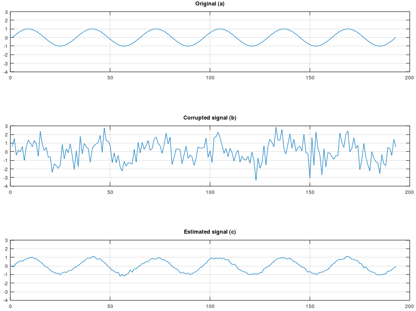
Top (a): Original desired signal
Middle (b): Corrupted signal
Bottom (c): Estimated signal using Wiener filter

Tell me in the comments other topics you find difficult and want a post on.

Practice Problems

This section contains practice problems to see if you know how to solve for the optimal coefficients.

Problem 1

Let $d(n)$ be the desired signal we wish to estimate and $x(n)$ be the noisy observation of $d(n)$ such that

$x(n) = d(n) + v(n)$

where $v(n)$ is white noise with $\sigma_v^2 =2$ . The noise $v(n)$ and desired signal $d(n)$ are uncorrelated. The first five values of the autocorrelation sequence are

$\bold{r}_d = [2, -1, 0.2, 0.5, 1.5]^T$ .

Solve for the optimal filter coefficients and compute the mean squared error.

Problem 2

Now assume that the design you are working on is highly resource intensive and you have been tasked with reducing the nonzero multiplies for the Wiener filter. Find the three optimal nonzero coefficients for the Wiener filter in problem 1.

Problem 3

Let the desired signal $d(n)$ be a first order autoregressive (AR(1)) process such that

$d(n) = 0.25d(n-1)+v(n)$

where $v(n)$ is white gaussian noise with zero mean and variance $\sigma^2 = 1$ . $v(n)$ is uncorrelated with $d(n-1)$ . Let $x(n)$ be the noisy observation of the desired signal such that

$x(n) = d(n)+z(n)$

where $z(n)$ is white Gaussian noise with zero mean and variance $\sigma^2 = 2.5$ . $z(n)$ uncorrelated with $d(n)$ . Calculate a five tap casual Wiener filter and compute the mean squared error.

Download Solutions

Christopher Hogstrom

christopher.hogstrom@grittyengineer.com

7 thoughts on “The optimal Causal FIR Wiener filter”

radarsat1 says:

April 28, 2019 at 5:34 pm

Sorry for my poor algebra skills, but in the part where you set the derivative to zero, how do you get from the second-to-last line to the last line? (Immediately before “Now that the derivative is set to zero”)

Reply
1. Christopher says:
  
  April 28, 2019 at 5:35 pm
  
  It’s a fair question and the first time I encountered something like it I was confused. Notice that we are taking the derivative with respect to w(k)*. The first term, d(n)*, goes away because it is not being multiplied by a weight. The second term is a summation of products produced by multiplying weights by samples of the observed signal. The summation variable is l (lower case L) which takes on a range of values from 0 to p-1. w(k)* is a single weight rather than a range of weights. When we take the derivative with respect to w(k)* the only term remaining is x*(n-k).
  
  Let me give an example. Exanding the summation we have
  
  w*(0)x*(n-0)+w*(1)x*(n-1)+w*(2)x*(n-2)…w*(p-1)x*(n-p+1). If I take the derivative with respect to w*(2) all that is left in the above sequence is x*(n-2).
  
  Does that help?
  
  Reply
  1. radarsat1 says:
    
    April 28, 2019 at 5:38 pm
    
    Oh I think I see, thank you. So the only term in that summation that changes with respect to w(k)* is x*(n-k), the rest become zero. This assumes that k<p, right? (But p being the length of the whole signal, this is obviously true.)
    
    Reply
    1. Christopher says:
      
      April 28, 2019 at 5:38 pm
      
      Yes, this assumes that k<p. P is actually the number of filter coefficients. The length of the signal could be infinite.
      
      Reply
      1. radarsat1 says:
        
        April 28, 2019 at 5:39 pm
        
        Ah right right, thanks!
Am king says:

April 5, 2020 at 7:42 pm

Thank you for your great post. I have a question :
Suppose that the noise was not white in Fig-1. Will the filter be able to remove the noise?
How to prove that it is optimal.

Reply
1. Christopher Hogstrom says:
  
  April 6, 2020 at 7:43 pm
  
  Thank you for your comment King. Yes, the filter will still be able to remove the noise. The challenge is to find the cross-correlation vector $\mathbf{r}_{dx}$ and the autocorrelation matrix $\mathbf{R}_x$ as shown in Equation 2. Aside from the fact that we started with minimizing the mean squared error, you can plug the solution back into the mean squared error and see what you get. You can also run some Monte Carlo simulations to empirically prove it to yourself. Hopefully, that helped and made sense. What other posts would you find interesting or would you like to see?
  
  Reply