In our last post, we went over active noise cancellation using the Wiener filter (you can find that here). It focused on using a single auxiliary sensor for active noise cancellation and while powerful there are cases when having multiple auxiliary sensors provides better noise reduction. Today’s example considers a car equipped with a hands-free phone call system. Such systems typically work by connecting the car’s microphone and speakers to a cell phone using Bluetooth. In many cases, it is assumed that the driver is the speaker and so the primary microphone is placed on the driver’s side dashboard, though sometimes it is placed inside the rearview mirror. While this location allows the sensor to pick up the speaker’s voice the microphone is likely to pick up unwanted noise generated by the car’s engine, outside wind, and the vibration of the tires going over the road. Such interference can make speech difficult to understand for listeners on the other end of the phone call.
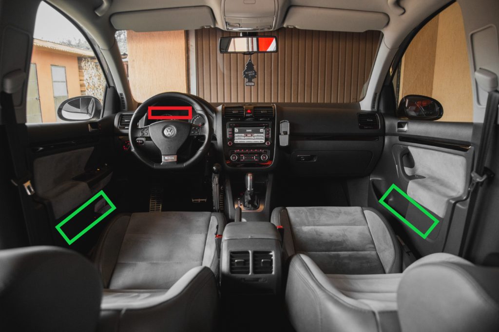
Active noise cancellation would sure be nice in this situation but where should we put the auxiliary sensor? We learned from the previous post that it must be located somewhere where it can pick up the interference but not the desired signal, the desired signal being speech in this example. Placing the auxiliary sensor in the car cabin will probably fail as it’s almost guaranteed that it will pick up the speaker’s voice. A better option is to put the auxiliary microphone inside the driver’s door. This way the microphone is able to pick up noise from the driver’s wheel well, engine noise, and wind noise. But noise is also coming from the passenger’s side and so we place an additional microphone inside the passenger’s door. Example placement is shown in Figure 1 where the red square indicates the potential location of the primary sensor and green indicates the potential locations of the auxiliary sensors.
While the microphones are trying to pick up noise generated by different sources (the different wheel wells and possibly wind blowing from one side or the other), they will also pick up interference generated by the same process (the engine noise). Because the two auxiliary sensors are correlated through the shared interference, independently using the active noise cancellation using a single sensor and iteratively estimating the signal is suboptimal. Instead, the correct approach is to derive the optimal weights to filter the auxiliary signals such that when the filtered auxiliary signals are jointly subtracted from the primary sensor only the desired signal remains.
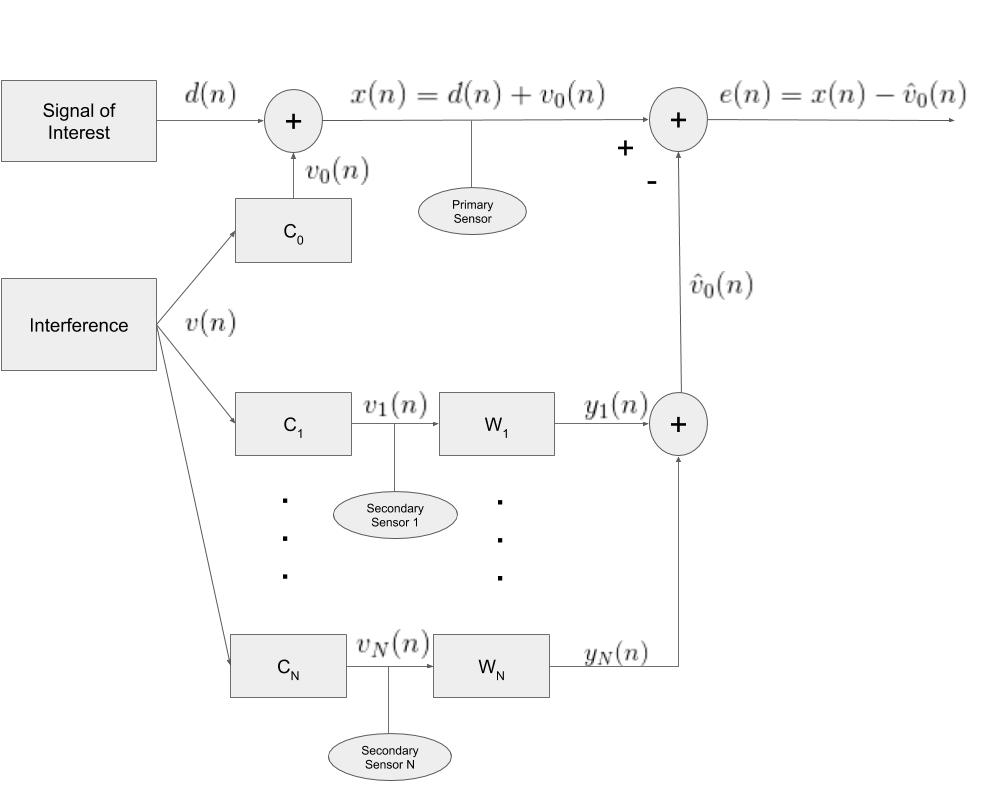
Figure 2 shows a block diagram of a generic active noise cancellation system using multiple auxiliary sensors.  represents the interference signal while the independent channel effects are modeled as filters. Channel effects are things such as propogation delays and distortion as the interference travels to each of the sensors. The optimal Wiener filters are represented as
  . Notice that the weights used to filter
  are different than the weights used to filter
  . Though the weights are unique they are solved for simultaneously.
Post Notations
Before going on to the derivation, let’s define some notation so that we’re all on the same page. Let  ,
,  and
and  represent the expectation operator, the estimate of
  , and the autocorrelation function of respectively. The expectation operator returns the expected value or mean of a random variable. The estimate of
  is found by combining the filtered auxiliary signals
  where
where  . is found by filtering
  with our Wiener filter as follows

where  is the number of filter coefficients.
The autocorrelation function for a wide sense stationary (WSS) signal is defined as
 .
.
The cross-correlation function for jointly WSS signals is defined as

Let the error be defined as the difference between the desired signal and the estimate of the desired signal

and the mean squared error (MSE) be defined as
 .
.
Finally, let  represent the complex conjugate operator.
Deriving the Active Noise-Canceling Wiener Filters
Using Figure 2 we now derive the active noise-canceling Wiener filters for multiple auxiliary signals. For this derivation, it is assumed that the signal of interest and the interference are jointly wide sense stationary. A signal is wide sense stationary if the signal has constant mean, the autocorrelation depends only on the lag, and the variance is finite. As defined in the above diagram the error is the corrupted signal minus the estimate of the interference.
Because we want to minimize the mean squared error we take the derivative of  with respect to
  and set it equal to zero.

Because the derivative of with respect to equals  the above equation simplifies to
![\begin{align*}0= E\{e v_q^*(n-k)\}\\0= E\{[x(n)-\hat{v}_0(n)] v_q^*(n-k)\}\\0= E\{x(n)v_q^*(n-k)-\hat{v}_0(n) v_q^*(n-k)\}\\0= E\{x(n)v_q^*(n-k)\}-E\{\hat{v}_0(n) v_q^*(n-k)\}\\E\{[y_1(n)+\dots+y_N(n)]v_q^*(n-k)\} = r_{xv_q}(k)\\E\{\sum_{\ell=0}^{p-1}w_1(\ell)v_1 (n-\ell)v_q^*(n-k) +\dots+\sum_{\ell=0}^{p-1}w_N(\ell)v_N (n-\ell) v_q^*(n-k)\} = r_{xv_q}(k)\\\sum_{\ell=0}^{p-1}w_1(\ell)E\{v_1 (n-\ell)v_q^*(n-k)\} +\dots+\sum_{\ell=0}^{p-1}w_N(\ell)E\{v_N (n-\ell) v_q^*(n-k)\} = r_{xv_q}(k)\\\sum_{\ell=0}^{p-1}w_1(\ell)r_{v_1 v_q} +\dots+\sum_{\ell=0}^{p-1}w_N(\ell)r_{v_N v_q} = r_{xv_q}(k)\\ \end{align*}](https://grittyengineer.com/wp-content/ql-cache/quicklatex.com-eee02bedbdf3a07a84d4311cab8de42c_l3.png "Rendered by QuickLaTeX.com")
We can write this in matrix-vector notation as

Or more genenerally as

Where

Multi Auxiliary Noise Cancellation Example
To hit home the power of using multiple auxiliary sensors I created a small audio example. The desired signal is corrupted by two noise sources, white noise, and a tone. To create the observed signal the white noise and tone are filtered by a first-order autoregressive filter before being added to the desired signal. The first auxiliary signal is created by filtering the white noise and tone by a different first-order autoregressive filter with the tone attenuated by 40 dB. The second auxiliary signal is created by filtering the white noise and tone by yet another first-order autoregressive filter but this time the white noise is attenuated by 40 dB.
Using the equations derived above, I computed the optimal noise-canceling Wiener filters and estimated the observed noise. Figure 3 plots the noise observed by the primary sensor, the noise observed by the auxiliary sensors and the estimate of the noise. The plot shows that each auxiliary sensor captures a different aspect of the interference. captures the filtered noise whereas  does a better job of capturing the filtered tone. From the figure, it can be a little hard to tell but
  lies nearly ontop of
  indicating a good estimate.
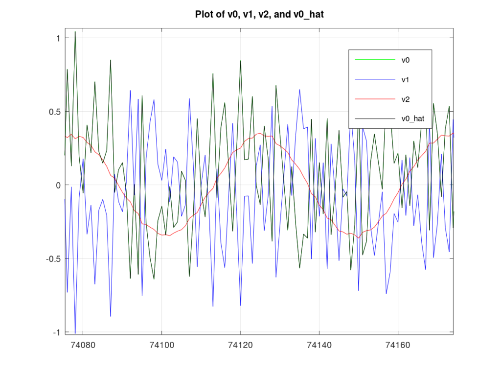
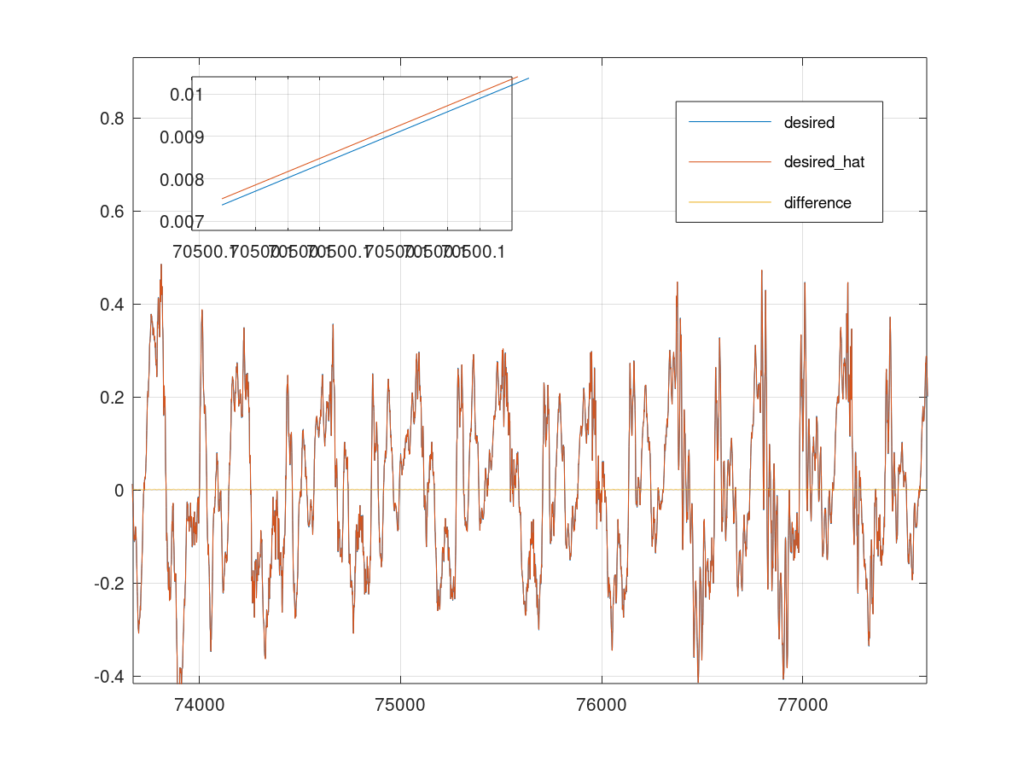
Figure 4 plots the desired signal and its estimate. It also plots the absolute difference between the desired signal and estimated signal. Once again, the estimate and desired signals lie nearly on top of each other and the difference between the two are minimal.
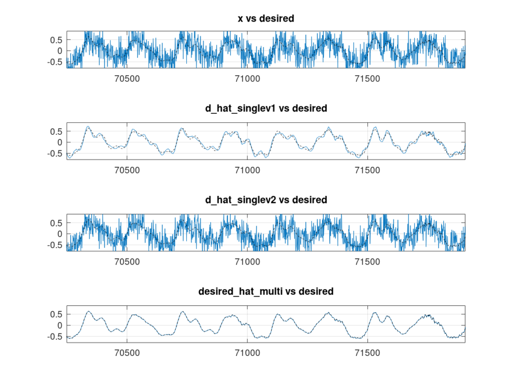
Using both auxiliary sensors is nice but how much better is it than just using one sensor? I decided to use just and just and come up with an estimate so that we could compare the performances. Figure 5 shows the results. When using just to form an estimate we get about 12 dB of improvement vs 5 dB of improvement when using . But when using both auxiliary sensors we get more than 45 dB of improvement! Before getting too excited, how much improvement you’ll see using multi-sensor noise-cancellation is dependent on many factors and will not always be so significant. For instance, if both and are essentially the same or contain highly redundant information then improvement will be limited.
Now that you’ve seen the difference see if you can hear the difference in the following audio clips. The first audio clip is the observed signal, the second is using single-sensor noise-cancellation using , followed by using only. The last audio clip uses the multi-sensor noise-cancellation system that we derived earlier. Notice that when canceling using only the tone is still very present in the audio clip. This makes sense as the tone was highly attenuated in . , on the other hand, does a great job cleaning up the tone but the white noise is still present for the same reason.
What happens if the desired signal is present on all sensors?
We’ve stated before that for active noise-cancellation to work the auxiliary sensors must be placed somewhere where it can pick up the noise signals but not the desired signals. But in some cases, it is not physically possible to make that happen. For instance, you might have a cochlear implant and wish background noise to be attenuated. Or you might be an astronomer picking up signals from space but interference from a nearby airplane is corrupting your data. These cases make it virtually impossible to have an auxiliary sensor dedicated to receiving the noise only signal. Lucky for us, we have one more trick up our sleeve that can still help us out. It’s called beamforming. We won’t go over it now but it’s a powerful tool that expands on our multi-sensor active noise-canceling system. Sign up for our newsletter to find out when we come out with our beamforming tutorial, it’s not something you’re going to want to miss out on.

Damn man this is exactly what I’ve been curious about these past few months. Awesome!
Aren’t these articles genius? I always wanted to know how this works.
Thanks! That was a really interesting read. I can’t wait for the next part.
Thanks, Nelieru! Is there anything that was unclear in the most or that could be improved? Aside from beamforming, which will be the next post I create, what other DSP topics would you be interested in learning about?
Honestly, no. It’s already pretty detailed and well explained. I had a bit of a hard time following the math buts that’s mostly due to my light math education lol. About the fields, I don’t really have an overview or general idea or what fields DSP are used in. So I guess all kind of topics were DSP are used in everyday life?
thanks,
really useful and interesting for me.